Exploring the CRAN social network
A few months ago, I published a post where I was trying to map the dependencies relationships between R packages. Today I want to do something similar with package contributors. My idea is to reconstruct a social graph where each node would be a person (presumably a developer), and two persons would be connected by an edge if they have collaborated on the same package. Thus I would be able to explore the CRAN social network!
This post is also a bit special for me. It’s the very first time I’m using dplyr and the tidyverse. I used to write my code in base R but the amazing work of Thomas Lin Pedersen around tiygraph and ggraph convinced me to take the plunge. And it was a lot of fun!
First, we load the packages and the data. In the first version of the project I used the XML file of each package that I retrieved from CRAN using wget and then read and parsed with xml2. Since R 3.4.0, things are much, much simpler with the function CRAN_package_db.
library(tidyverse)
library(stringr)
library(igraph)
library(tidygraph)
library(ggraph)
library(magrittr)

pdb <- tools::CRAN_package_db()
aut <- pdb$Author
That’s all we need to get the full list of contributors. But it comes in a very messy way. R provides a structured system to describe persons which should be used in the Authors@R field of the DESCRIPTION file, but most people use a simple character string.
The big cleanup
I combined a series of regular expressions and string manipulations to extract every name. It was the first time I was using stringr and I have to say, I don’t regret gsub, grepl, etc. I just miss the support for some PCRE functionalities…
aut <- aut %>%
  str_replace_all("\\(([^)]+)\\)", "") %>%
  str_replace_all("\\[([^]]+)\\]", "") %>%
  str_replace_all("<([^>]+)>", "") %>%
  str_replace_all("\n", " ") %>%
  str_replace_all("[Cc]ontribution.* from|[Cc]ontribution.* by|[Cc]ontributors", " ") %>%
  str_replace_all("\\(|\\)|\\[|\\]", " ") %>%
  iconv(to = "ASCII//TRANSLIT") %>%
  str_replace_all("'$|^'", "") %>%
  gsub("([A-Z])([A-Z]{1,})", "\\1\\L\\2", ., perl = TRUE) %>%
  gsub("\\b([A-Z]{1}) \\b", "\\1\\. ", .) %>%
  map(str_split, ",|;|&| \\. |--|(?<=[a-z])\\.| [Aa]nd | [Ww]ith | [Bb]y ", simplify = TRUE) %>%
  map(str_replace_all, "[[:space:]]+", " ") %>%
  map(str_replace_all, " $|^ | \\.", "") %>%
  map(function(x) x[str_length(x) != 0]) %>%
  set_names(pdb$Package) %>%
  extract(map_lgl(., function(x) length(x) > 1))

aut_list <- aut %>%
  unlist() %>%
  dplyr::as_data_frame() %>%
  count(value) %>%
  rename(Name = value, Package = n)
At this point we have a list of 13668 (unique) names, and this number is increasing almost every day. The R community is huge! Of course there are still some errors. And we can find surprising contributors:
aut_list$Name[4922]
# [1] "Her Majesty the Queen in Right of Canada"
The Social Network
The next step is to produce a two-column matrix describing all the connections of the network (edge list). An edge list can be turned into a graph object with the igraph package. Finally we can convert the igraph graph into a tidy graph so we can use the API provided by the tidygraph package. For example to filter nodes/edges or select only the main component.
edge_list <- aut %>%
  map(combn, m = 2) %>%
  do.call("cbind", .) %>%
  t() %>%
  dplyr::as_data_frame() %>%
  arrange(V1, V2) %>%
  count(V1, V2)

g <- edge_list %>%
  select(V1, V2) %>%
  as.matrix() %>%
  graph.edgelist(directed = FALSE) %>%
  as_tbl_graph() %>%
  activate("edges") %>%
  mutate(Weight = edge_list$n) %>%
  activate("nodes") %>%
  rename(Name = name) %>%
  mutate(Component = group_components()) %>%
  filter(Component == names(table(Component))[which.max(table(Component))])
The author of tidygraph, Thomas, also developed the ggraph package, an implementation of the grammar of graphics for relational data. Using ggraph, it is very easy to visualize our graph.
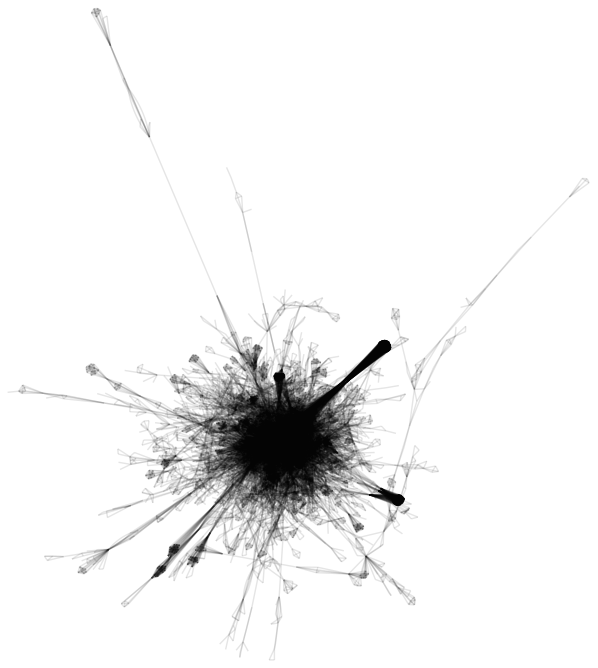
ggraph(g, layout = 'lgl') +
  geom_edge_fan(alpha = 0.1) +
  theme_graph()
This is it! This hairy ink stain is the main connected component of the CRAN social network, representing collaborations between 6758 developers!
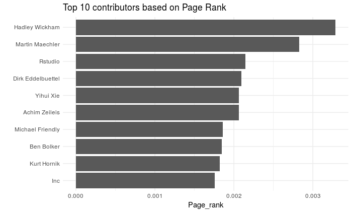
We can look for who’s the « most important » node in the graph according to the Google’s PageRank algorithm, although it’s not straightforward what could mean a high PR here…
g %>%
  mutate(Page_rank = centrality_pagerank()) %>%
  top_n(10, Page_rank) %>%
  as_tibble() %>%
  ggplot() +
    geom_col(aes(forcats::fct_reorder(Name, Page_rank), Page_rank)) +
    coord_flip() + theme_minimal() +
    labs(title = "Top 10 contributors based on Page Rank", x = "")
Focus on the core network
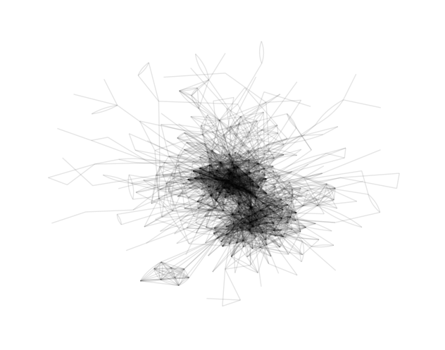
The complete graph makes a nice painting to hang on the wall of your living room. But hard to say anything about it. So, we will reduce the data and focus on the contributors involved in more than 4 packages.
g <- g %>%
  left_join(aut_list) %>%
  filter(Package > 4) %>%
  mutate(Component = group_components()) %>%
  filter(Component == names(table(Component))[which.max(table(Component))])

ggraph(g, layout = 'lgl') +
  geom_edge_fan(alpha = 0.1) +
  theme_graph()
Nice! It seems like there are two distinct clusters in the middle. Let’s see if we can identify them using a community detection algorithm.
g <- mutate(g, Community = group_edge_betweenness(),
            Degree = centrality_degree())

filter(g, Community == names(sort(table(Community), decr = TRUE))[1]) %>%
  select(Name, Package) %>%
  arrange(desc(Package)) %>%
  top_n(10, Package) %>%
  as_tibble() %>%
  knitr::kable(format = "html", caption = "Cluster 1")
filter(g, Community == names(sort(table(Community), decr = TRUE))[2]) %>%
  select(Name, Package) %>%
  arrange(desc(Package)) %>%
  top_n(10, Package) %>%
  as_tibble() %>%
  knitr::kable(format = "html", caption = "Cluster 2")
| Name | Package |
|---|---|
| Kurt Hornik | 56 |
| Martin Maechler | 46 |
| Achim Zeileis | 44 |
| Dirk Eddelbuettel | 41 |
| Romain Francois | 27 |
| Ben Bolker | 25 |
| Brian Ripley | 25 |
| Torsten Hothorn | 24 |
| Roger Bivand | 23 |
| Douglas Bates | 23 |
| Name | Package |
|---|---|
| Hadley Wickham | 95 |
| Rstudio | 92 |
| Scott Chamberlain | 44 |
| Inc | 36 |
| Yihui Xie | 34 |
| Jeroen Ooms | 33 |
| Jj Allaire | 29 |
| R. Core Team | 27 |
| Bob Rudis | 26 |
| Gabor Csardi | 22 |
| Oliver Keyes | 22 |
| Winston Chang | 22 |
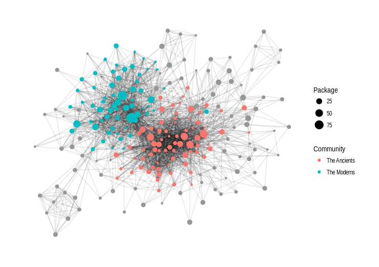
If you know a bit R and its community, you will certainly recognize some names. The challenge is to interpret this classification. It is not a good thing to put people in boxes, but this is mandatory to make nice and colorful visualizations! So, I give it a try. For me, the first group include people of the early days who contributed to major packages which constitute the heart of R. The second group is more related to the second generation, associated with Rstudio products and who have been particularly prolific in the last years. Of course the two groups are strongly connected.
How can we label these two groups? After long consideration, I chose to go for « The Ancients » and « The Moderns », without any value judgment! This is a reference to an old debate in French literature. This dubious comparison would certainly be more appropriate to designate the ongoing debate base vs. tidyverse, but… not today!
Let’s see how we can visualize these two groups.
g <- g %>%
  mutate(Community = case_when(Community == names(sort(table(Community),
                                                       decr = TRUE))[1] ~ "The Ancients",
                               Community == names(sort(table(Community),
                                                       decr = TRUE))[2] ~ "The Moderns",
                               Community %in% names(sort(table(Community),
                                                       decr = TRUE))[-1:-2] ~ "Unclassified")) %>%
  mutate(Community = factor(Community))

g <- g %>%
  filter(Degree > 5) %>%
  mutate(Degree = centrality_degree())

ggraph(g, layout = 'lgl') +
  geom_edge_fan(alpha = 0.1) +
  geom_node_point(aes(color = Community, size = Package)) +
  theme_graph() +
  scale_color_manual(breaks = c("The Ancients", "The Moderns"),
                     values=c("#F8766D", "#00BFC4", "#969696"))
ggraph really does a great job! I really like the result.
BTW, the R community is not really divided…
g %>% activate("edges") %>%
  mutate(Community_from = .N()$Community[from],
         Community_to = .N()$Community[to]) %>%
  filter((Community_from == "The Ancients" & Community_to == "The Moderns")|
           Community_from == "The Moderns" & Community_to == "The Ancients") %>%
  as_tibble() %>%
  nrow()
… there are 254 edges connecting the the Ancients and the Moderns! But I think this is a nice illustration of how social graphs keeps the imprint of history and past events. Next step would be to look at the graph dynamics over time. Maybe an idea for a future post…

5 réactions au sujet de « Exploring the CRAN social network »
This is an interesting analysis indeed! The top beautiful figure is quite similar to an oriental painting style. So artistic.
Thanks so much for the nice post! 😀
Thank you very much for this great post.
I’d like to stress that I only have ~ 6 months of experience in R, so going through the post however I encountered a couple of issues.
First of all, running blindly the « big cleanup » I obtained the following error:
Error in parse(text = dbname) : :1:7: unexpected symbol
1: Scott Fortmann
^
Then, going through the single steps I found out that I am unable to interpret the following regex: « \\[([^]]+)\\] ». I looked for solutions in https://regexr.com/ but to no avail.
Hi Florian, I’m afraid I have no idea why it is not working for you. I tried again and it works on my computer, the syntax of this regex is correct. Hope you can find a solution.
Hi Francois,
Thanks a lot for your answer. I will keep investigating. 🙂